44 how to add data labels to a pie chart in excel

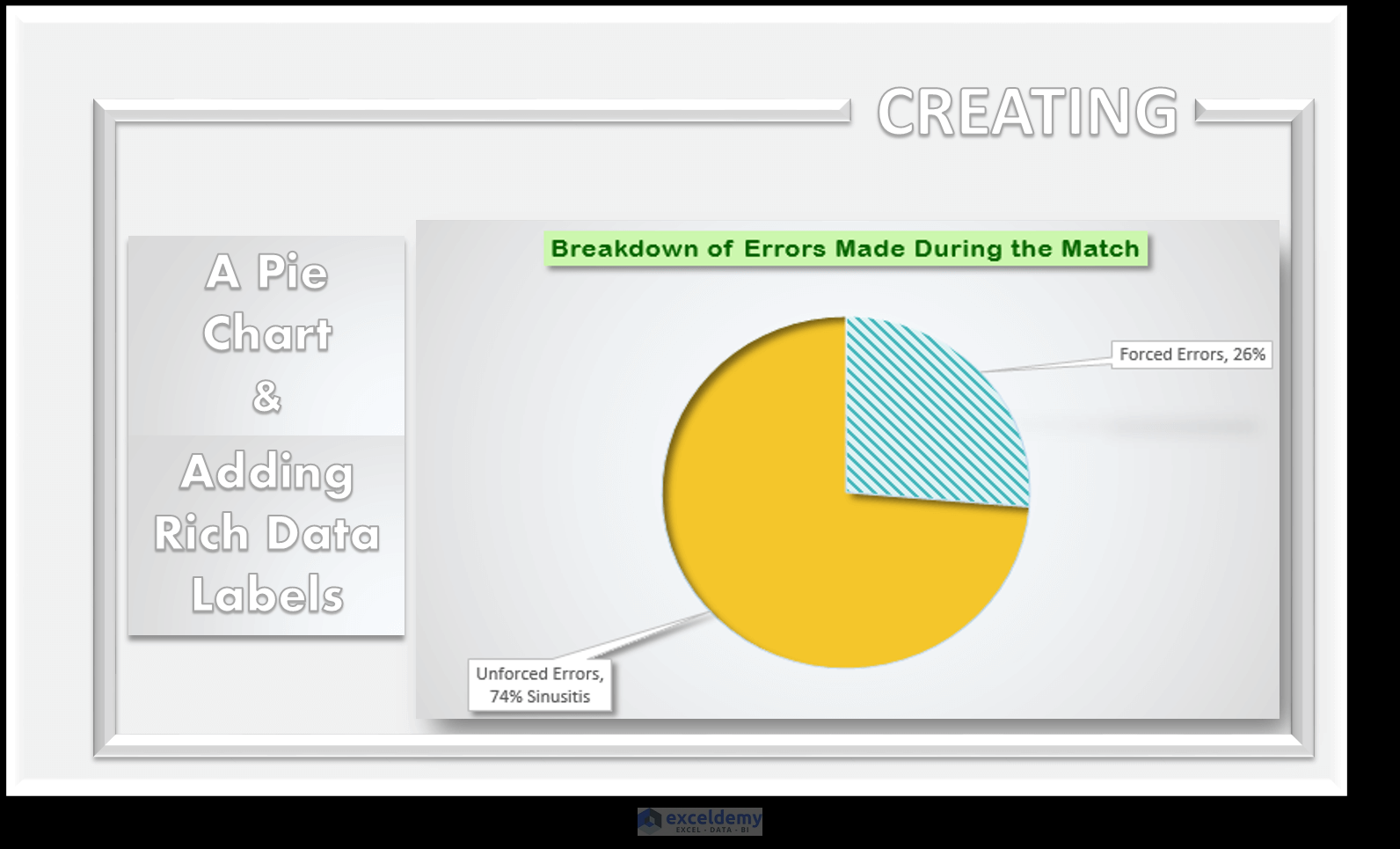
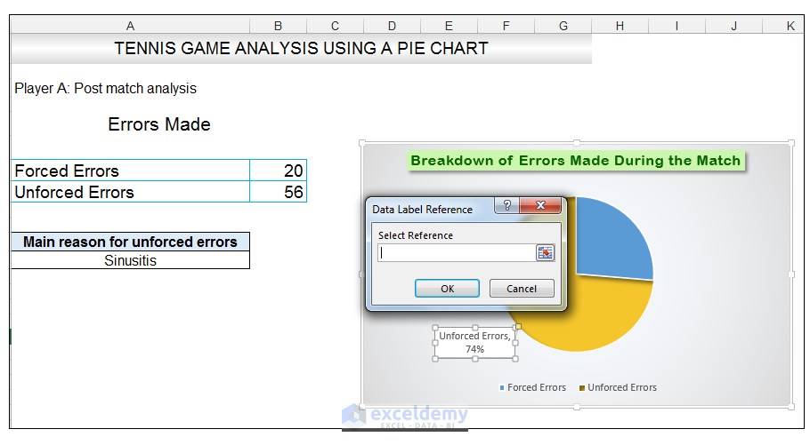
How to Make a Pie Chart in Excel & Add Rich Data Labels to ... Formatting the Data Labels of the Pie Chart 1) In cell A11, type the following text, Main reason for unforced errors, and give the cell a light blue fill and a black border. 2) In cell A12, type the text Sinusitis, and give the cell a black border, and align the text to the center position. Doughnut Chart in Excel | How to Create Doughnut Chart in ... Select the data table and click on the Insert menu. Under charts, select the Doughnut chart. The chart will look like below. Now click on the + symbol that appears top right of the chart, which will open the popup. Untick the Chart Title and Legend to remove the text in the chart.

How to Create A 3-D Pie Chart in Excel [FREE TEMPLATE] The data in the table is pretty self-explanatory, so move on to the nitty-gritty. Here's the easiest way to create a 3-D pie chart: Select any cell in the data table ( A1:A6 ). Switch to the Insert tab. Choose " Insert Pie or Doughnut Chart. ". Click " 3-D Pie. ". Just a few clicks are your 3-D chart is ready to go:

How to add data labels to a pie chart in excel

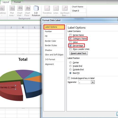
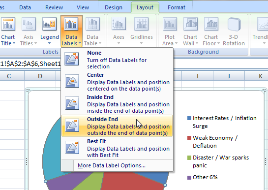
How to Create a Pie Chart in Excel - Smartsheet If want the category names to appear on or near the chart, right-click on the chart and click Add Data Labels …. By default, the numerical values are added. To add other labels, such as the categorical values or the percentage of the total that each category represents, right-click on the chart, then click Format Data Labels …. How to display leader lines in pie chart in Excel? To display leader lines in pie chart, you just need to check an option then drag the labels out. 1. Click at the chart, and right click to select Format Data Labels from context menu. 2. In the popping Format Data Labels dialog/pane, check Show Leader Lines in the Label Options section. See screenshot: 3. Possible to add second data label to pie chart? Re: Possible to add second data label to pie chart? Create the composite label in a worksheet column by concatenating the data in other cells and the nextline character, CHR (10). Now, use this composite label column as the source for Rob Bovey's add-in. -- Regards, Tushar Mehta Excel, PowerPoint, and VBA add-ins, tutorials

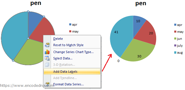
How to add data labels to a pie chart in excel. Add a Data Callout Label to Charts in Excel 2013 ... The new Data Callout Labels make it easier to show the details about the data series or its individual data points in a clear and easy to read format. How to Add a Data Callout Label. Click on the data series or chart. In the upper right corner, next to your chart, click the Chart Elements button (plus sign), and then click Data Labels. Excel charts: add title, customize chart axis, legend and ... To add a label to one data point, click that data point after selecting the series. Click the Chart Elements button, and select the Data Labels option. For example, this is how we can add labels to one of the data series in our Excel chart: For specific chart types, such as pie chart, you can also choose the labels location. How to Create and Format a Pie Chart in Excel - Lifewire To add data labels to a pie chart: Select the plot area of the pie chart. Right-click the chart. Select Add Data Labels . Select Add Data Labels. In this example, the sales for each cookie is added to the slices of the pie chart. Change Colors ☝️How to Create a Pie Chart in Excel (Free Template ... To make our circle chart a bit more informative, add some data labels illustrating the numeric value of each slice by right-clicking on your pie chart and choosing "Add Data Labels. Once there, Excel will automatically generate dynamic data labels based on your actual values.

Video: Insert a pie chart Quickly add a pie chart to your presentation, and see how to arrange the data to get the result you want. Customize chart elements, apply a chart style and colors, and insert a linked Excel chart. Add a pie chart to a presentation in PowerPoint. Use a pie chart to show the size of each item in a data series, proportional to the sum of the items. Pie of Pie Chart in Excel - Inserting, Customizing - Excel ... To add the data labels:- Select the chart and click on + icon at the top right corner of chart. Mark the check box containing data labels. Formatting Data Labels Consequently, this is going to insert default data labels on the chart. How to show percentage in pie chart in Excel? Select the data you will create a pie chart based on, click Insert > I nsert Pie or Doughnut Chart > Pie. See screenshot: 2. Then a pie chart is created. Right click the pie chart and select Add Data Labels from the context menu. 3. Now the corresponding values are displayed in the pie slices. Inserting Data Label in the Color Legend of a pie chart ... Re: Inserting Data Label in the Color Legend of a pie chart @SabrinaFr There is no built-in way to do that, but you can use a trick: see Add Percent Values in Pie Chart Legend (Excel 2010)

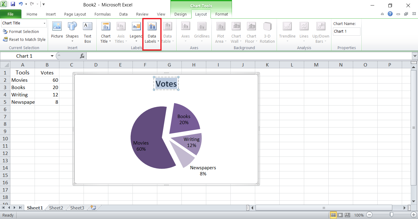
Free Pie Chart Maker - Make Your Own Pie Chart | Visme To use the pie chart maker, click on the data icon in the menu on the left. Enter the Graph Engine by clicking the icon of two charts. Choose the pie chart option and add your data to the pie chart creator, either by hand or by importing an Excel or Google sheet. Microsoft Excel Tutorials: Add Data Labels to a Pie Chart The chart is selected when you can see all those blue circles surrounding it. Now right click the chart. You should get the following menu: From the menu, select Add Data Labels. New data labels will then appear on your chart: The values are in percentages in Excel 2007, however. To change this, right click your chart again. How to Use Cell Values for Excel Chart Labels Select the chart, choose the "Chart Elements" option, click the "Data Labels" arrow, and then "More Options." Uncheck the "Value" box and check the "Value From Cells" box. Select cells C2:C6 to use for the data label range and then click the "OK" button. The values from these cells are now used for the chart data labels. How to show data labels in charts created via Openpyxl ... Data labels are set per chart, per series or even per item within a series. At the moment you'll have to look at the source and work out how this works but chart.dataLabels or chart.series[0].label is the place to start.

How to Create a Pie Chart in Excel using Worksheet Data

Multiple data labels (in separate locations on chart) Running Excel 2010 2D pie chart I currently have a pie chart that has one data label already set. The Pie chart has the name of the category and value as data labels on the outside of the graph. I now need to add the percentage of the section on the INSIDE of the graph, centered within the pie section. I'm aware that I could type in the percentages as text boxes, but I want this graph to ...

Data labels on Excel charts « projectwoman.com

How To Add and Remove Legends In Excel Chart? - EDUCBA A Legend is a representation of legend keys or entries on the plotted area of a chart or graph, which are linked to the data table of the chart or graph. By default, it may show on the bottom or right side of the chart. The data in a chart is organized with a combination of Series and Categories. Select the chart and choose filter then you will ...

How to Make a Pie Chart in Excel & Add Rich Data Labels to The Chart!

Add data labels and callouts to charts in Excel 365 ... The steps that I will share in this guide apply to Excel 2021 / 2019 / 2016. Step #1: After generating the chart in Excel, right-click anywhere within the chart and select Add labels . Note that you can also select the very handy option of Adding data Callouts.

Create A Pie Chart In Excel With and Easy Step-By-Step Guide

Display data point labels outside a pie chart in a ... Create a pie chart and display the data labels. Open the Properties pane. On the design surface, click on the pie itself to display the Category properties in the Properties pane. Expand the CustomAttributes node. A list of attributes for the pie chart is displayed. Set the PieLabelStyle property to Outside. Set the PieLineColor property to Black.

How to Create and modify a pie chart in Excel | HowTech

Create Pie Chart In Excel - PieProNation.com Show percentage in pie chart in Excel. Please do as follows to create a pie chart and show percentage in the pie slices. 1. Select the data you will create a pie chart based on, click Insert> Insert Pie or Doughnut Chart> Pie. See screenshot: 2. Then a pie chart is created. Right click the pie chart and select Add Data Labels from the context ...

How to Make a Pie Chart in Excel & Add Rich Data Labels to The Chart!

Add data labels to excel pie chart - Stack Overflow Add data labels to excel pie chart. Ask Question Asked 9 years, 8 months ago. Modified 5 years, 9 months ago. Viewed 9k times 4 1. I am drawing a pie chart with some data: private void DrawFractionChart(Excel.Worksheet activeSheet, Excel.ChartObjects xlCharts, Excel.Range xRange, Excel.Range yRange) { Excel.ChartObject myChart = (Excel ...

ExcelSirJi | Excel Data Tips | How to Create Pie Chart in Excel (Complete Tutorial) ExcelSirJi

Add or remove data labels in a chart Click the data series or chart. To label one data point, after clicking the series, click that data point. In the upper right corner, next to the chart, click Add Chart Element > Data Labels. To change the location, click the arrow, and choose an option. If you want to show your data label inside a text bubble shape, click Data Callout.

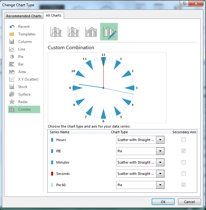
Building an Excel Clock Chart - Xcelanz

Pie Chart in Excel | How to Create Pie Chart | Step-by ... Step 1: Do not select the data; rather, place a cursor outside the data and insert one PIE CHART. Go to the Insert tab and click on a PIE. Step 2: once you click on a 2-D Pie chart, it will insert the blank chart as shown in the below image. Step 3: Right-click on the chart and choose Select Data.

How to Make a Pie Chart in Excel & Add Rich Data Labels to The Chart!

Office: Display Data Labels in a Pie Chart 2. If you have not inserted a chart yet, go to the Insert tab on the ribbon, and click the Chart option. 3. In the Chart window, choose the Pie chart option from the list on the left. Next, choose the type of pie chart you want on the right side. 4. Once the chart is inserted into the document, you will notice that there are no data labels.

Excel rotate radar chart - Stack Overflow

Edit titles or data labels in a chart - support.microsoft.com On a chart, click one time or two times on the data label that you want to link to a corresponding worksheet cell. The first click selects the data labels for the whole data series, and the second click selects the individual data label. Right-click the data label, and then click Format Data Label or Format Data Labels.

How to Make a Pie Chart in Excel & Add Rich Data Labels to The Chart!

How to Create Pie Charts in Excel (In Easy Steps) Select the pie chart. 9. Click the + button on the right side of the chart and click the check box next to Data Labels. 10. Click the paintbrush icon on the right side of the chart and change the color scheme of the pie chart. Result: 11. Right click the pie chart and click Format Data Labels. 12.

Charts In Excel – Excel Tutorial World

Excel: How to not display labels in pie chart that are 0% ... I have some data in excel that I want to graph in a pie chart (see image 1) where the text will be the labels and the numbers will turn into percentages. The problem is, when i go to graph the data...

How-to Make a WSJ Excel Pie Chart with Labels Both Inside and Outside - Excel Dashboard Templates

Possible to add second data label to pie chart? Re: Possible to add second data label to pie chart? Create the composite label in a worksheet column by concatenating the data in other cells and the nextline character, CHR (10). Now, use this composite label column as the source for Rob Bovey's add-in. -- Regards, Tushar Mehta Excel, PowerPoint, and VBA add-ins, tutorials

Pie Charts Solution | ConceptDraw.com

How to display leader lines in pie chart in Excel? To display leader lines in pie chart, you just need to check an option then drag the labels out. 1. Click at the chart, and right click to select Format Data Labels from context menu. 2. In the popping Format Data Labels dialog/pane, check Show Leader Lines in the Label Options section. See screenshot: 3.